
Achieving CartPole Environment Solution via DQN within One Second
Advancements in Reinforcement Learning (RL) have seen remarkable strides, exemplified by Waymo’s self-driving taxis and DeepMind’s exceptional chess-playing agents.

These advancements integrate classical RL with Deep Learning elements like Neural Networks and Gradient Optimization methods.
Expanding on earlier concepts and coding principles, this exploration delves into Deep Q-Networks (DQN) and replay buffers for solving OpenAI’s CartPole environment. All achieved within a second using JAX!
Deep Reinforcement Learning using JAX
This piece will encompass the following segments:
The Importance of Deep RL
Deep Q-Networks: Theory and Application
Understanding Replay Buffers
Adapting the CartPole Environment to JAX
Efficient Training Loop Implementation with JAX
The Importance of Deep RL
The necessity for Deep RL stems from the limitations of Q-learning, an off-policy algorithm managing a Q-table that maps states to respective action values.
While Q-learning suits scenarios with discrete action and limited observation spaces, its adaptability weakens in complex environments.
The challenge lies in crafting a comprehensive Q-table, especially evident in autonomous driving. Here, the observation space comprises infinite potential configurations from sensor inputs, while the action space spans various steering and vehicle control options.
Despite the potential to discretize the action space, the vast array of possible states and actions makes an operational Q-table impractical in real-world applications.
To navigate extensive and intricate state-action spaces effectively, robust function approximation algorithms are essential. Neural Networks serve this purpose in Deep Reinforcement Learning, substituting the Q-table and effectively addressing the challenge of high-dimensional state spaces.
Additionally, explicit definition of the observation space becomes unnecessary.
DQN employs two neural networks simultaneously: the “online” network predicts Q-values and aids decision-making, while the “target” network generates stable Q-targets, evaluating the online network’s performance through the loss function.
Similar to Q-learning, DQN agents are characterized by two functions: act and update.
The act function executes an epsilon-greedy policy based on the estimated Q-values from the online neural network. Essentially, the agent chooses the action associated with the highest predicted Q-value for a specific state, sometimes opting for random actions based on a pre-set probability.
Unlike Q-learning, which updates its Q-table after each step, Deep Learning commonly employs batch-based updates through gradient descent.
Consequently, DQN utilizes a replay buffer to store experiences (comprising state, action, reward, next_state, done_flag tuples).
During network training, batches of experiences are sampled from this buffer instead of solely relying on the most recent experience. Further details are elaborated in the Replay Buffer section.
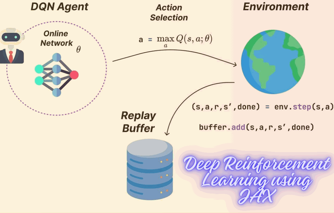
Here is an implementation in JAX for the action-selection segment of DQN:

One key aspect of this snippet is that unlike typical frameworks like PyTorch or TensorFlow, the model attribute doesn’t contain internal parameters.
In this context, the model represents a function simulating a forward pass through our architecture. However, the mutable weights are stored externally and passed as arguments.
This clarifies why we can utilize jit while marking the self argument as static, considering the model as stateless compared to other class attributes.
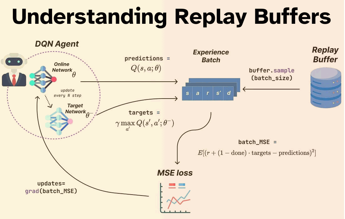
The update function’s role is to train the network by calculating a mean squared error (MSE) loss derived from the temporal-difference (TD) error:

The loss function employs θ to represent the parameters of the online network and θ− for the parameters of the target network. Updating the target network’s parameters from the online network’s parameters occurs every N steps, acting akin to a checkpoint (N is a hyperparameter).
This separation of parameters (θ for current Q-values and θ− for target Q-values) plays a critical role in ensuring training stability.
Using identical parameters for both would resemble targeting a moving object, where network updates promptly alter the target values.
Periodically refreshing θ− (freezing these parameters for a specified number of steps) maintains stable Q-targets, allowing the online network to continue learning.
Additionally, the (1-done) term adjusts the target for terminal states. When an episode concludes (i.e., ‘done’ equals 1), there exists no subsequent state. Hence, the Q-value for the next state is set to 0.
The update function in DQN entails a slightly more intricate process, let’s dissect it:
Firstly, the _loss_fn function is responsible for implementing the previously described squared error for an individual experience.
Following that, _batch_loss_fn serves as a wrapper for _loss_fn and incorporates vmap, applying the loss function to a batch of experiences. Subsequently, the average error for this batch is returned.
Lastly, the update function functions as the final layer to our loss function. It computes the gradient concerning the online network parameters, the target network parameters, and a batch of experiences.
Utilizing Optax (a commonly used JAX library for optimization), it executes an optimizer step, updating the online parameters.
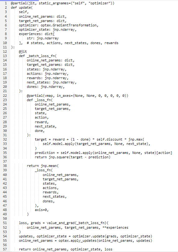
The code exhibits a principle where the model and optimizer are pure functions, altering an external state. The subsequent line exemplifies this concept:
updates, optimizer_state = optimizer.update(grads, optimizer_state)That’s why a single model serves both the online and target networks, allowing external storage and updates of parameters.
# target network predictions
self.model.apply(target_net_params, None, state)
# online network predictions
self.model.apply(online_net_params, None, state)
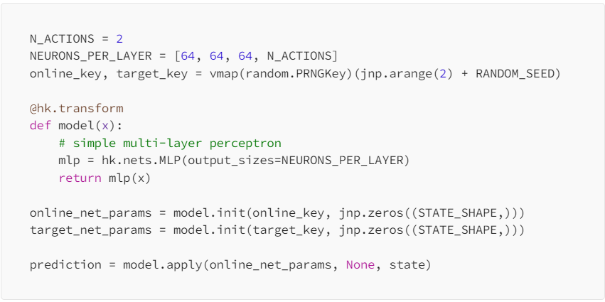
In this context, the model utilized in this edition is a multi-layer perceptron, outlined as follows:
“Let’s take a closer look at replay buffers. In reinforcement learning, they serve multiple purposes:
- Generalization: By sampling experiences from the buffer, we disrupt the correlation between consecutive events. This helps prevent overfitting to specific experience sequences.
- Diversity: As sampling isn’t restricted to recent events, it reduces variance in updates, avoiding overfitting to the latest experiences.
- Enhanced sample efficiency: Repeated sampling of experiences allows the model to learn more from individual encounters.”
“Various sampling schemes can be utilized for the replay buffer:
- Uniform sampling: Experiences are randomly sampled, allowing the model to learn from experiences independently of their collection time.
- Prioritized sampling: This category encompasses algorithms like Prioritized Experience Replay (PER, Schaul et al. 2015) or Gradient Experience Replay (GER, Lahire et al., 2022). These methods prioritize experience selection based on metrics associated with their ‘learning potential,’ such as the amplitude of the TD error for PER or the norm of the experience’s gradient for GER.”
“For simplicity, we’ll focus on implementing a uniform replay buffer in this article. However, I aim to delve deeper into prioritized sampling in future discussions.
The implementation of a uniform replay buffer is relatively straightforward, yet it involves certain intricacies when using JAX and functional programming. As per JAX’s requirements for constant-sized arrays in jit-compiled code to XLA, we initialize a buffer_state dictionary.
This dictionary maps keys to empty arrays with predefined shapes since we cannot define the buffer as a class instance with internal variable states, maintaining pure functions devoid of side effects.”

We utilize a Uniform Replay Buffer class to manage interactions with the buffer state. This class incorporates two primary methods:
add: Unpacks an experience tuple and associates its components with a specific index. To ensure proper functionality when the buffer reaches capacity, idx = idx % self.buffer_size ensures that new experiences overwrite older ones.
sample: Randomly selects a sequence of indexes from a uniform distribution. The sequence length, determined by batch_size, ranges from [0, current_buffer_size-1].
This prevents sampling from empty arrays while the buffer is not yet full. Leveraging JAX’s vmap in conjunction with tree_map, it returns a batch of experiences.

“We’ll now create a vectorized CartPole environment using the same framework. CartPole is a control environment with a substantial continuous observation space, providing an excellent testbed for evaluating our DQN agent.”

The process is fairly simple: we utilize most of OpenAI’s Gym implementation while ensuring the utilization of JAX arrays and lax control flow rather than Python or Numpy alternatives.

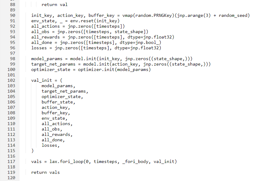
The final segment of our DQN setup is the training loop, often referred to as the rollout. Adhering to a specific structure is crucial to leverage JAX’s efficiency.
Although the rollout function might seem intricate initially, most of its intricacies are essentially related to syntax, considering we’ve already discussed the fundamental components. Here’s a step-by-step pseudo-code guide:
– Create empty arrays to hold states, actions, rewards, and done flags for each timestep. Initialize the networks and optimizer using placeholder arrays.
– Bundle all initialized objects into a value tuple.
– Unpack the value tuple.
– (Optional) Decay epsilon using a decay function.
– Take an action based on the state and model parameters.
– Execute an environment step and observe the next state, reward, and done flag.
– Form an experience tuple (state, action, reward, new_state, done) and add it to the replay buffer.
– Sample a batch of experiences based on the current buffer size (e.g., sample only from experiences with non-zero values).
– Update the model parameters using the experience batch.
– Every N steps, update the target network’s weights (set target_params = online_params).
– Store the experience values for the current episode and return the updated `value` tuple.


“Running DQN for 20,000 steps shows promising performance. It takes roughly 45 episodes for the agent to achieve decent results, consistently balancing the pole for over 100 steps.
The green bars mark instances where the agent successfully balanced the pole for over 200 steps, effectively solving the environment. Notably, the agent hit its peak performance on the 51st episode, maintaining balance for 393 steps.”

The training of 20,000 steps completed in slightly over a second, achieving an impressive pace of 15,807 steps per second on a single CPU!
This swift performance underscores JAX’s remarkable scalability, enabling practitioners to conduct extensive parallel experiments with minimal hardware demands.
Running for 20,000 iterations: 100%|██████████| 20000/20000 [00:01<00:00, 15807.81it/s]
“We’ll delve into parallelized rollout procedures for conducting statistically significant experiments and exploring hyperparameters in an upcoming edition!”
Conclusion
“Thanks for sticking around till the end! I hope this edition gave you a good start in Deep RL using JAX. If you have any questions or feedback about the content, feel free to reach out. I’m always here for a chat!”
“See you next time! 👋”
Get Access all prompts: https://bitly.com/machinelearning